• Algos

    Pairs Trading: The Math behind the Code

    Over the past several years, I have experimented with different programming languages (Python, R, GNU Octave and Matlab) to implement facets of quantitative trading techniques. Personally, I have found this very fulfilling because it brings together three disciplines that interest me – finance, programming and math – in no particular order. The rubric of this process has evolved over several years and I have had to course correct and go back to the drawing board often. Since some of the actual code has been used in a commercial interest, I want to heed respect to any such obligation and refrain from using prop code in this blog. However, I have also come to realize that the code in and of itself (or the programming language) is only of secondary importance. What really matters is an appreciation of the mathematical principles underlying the trading strategy and a good disposition to risk management. My strong sense is that many of these core concepts can be applied in a health care data analysis setting; without codifying everything under the hard label of AI/ML.

    The usage of different programming languages was mostly curiosity in terms of feature sets laid out in each and I have gravitated towards open source when possible. However, for this example below specific to Pairs Trading, I have used snippets of Matlab code for efficiency purposes. PS: I do wish GNU Octave had an elegant implementation of the Augmented Dickey Fuller test which I use below in Matlab.


    What is Pairs Trading?

    Pairs trading is a market neutral strategy (i.e. theoretically a trading strategy if constructed correctly can provide excess returns irrespective of a broader up/down/sideways market). This makes it, at least on the surface, an appealing hedge strategy. However, there is plenty of academic and market research that suggests that calls into question the efficacy of such a strategy. In my opinion the failures could be primarily due to the following reasons:

    1) Picking the wrong assets to pairs trade. A cursory instinct is to pick firms that seem to be operating in the space space ( eg, (Pepsi, Coca Cola), (Intel, AMD), (Home Depot, Lowes), (Analog Devices, Maxim Integrated) etc to go into a pairs trade. However, without really analyzing and back-testing relevant data attributed to these pairs, the trading strategy may not achieve its objective. 

    2) Very poor testing strategy accentuated by complicated models and data snooping. Very often, quantitatively oriented market participants have a tendency to deploy overly parameterized and therefore complicated models. Parameters are added on to just prove a preconceived notion

    3) Wrong duration. A certain strategy may work only for a specific time period. Extrapolating those results to a different duration ( or going out of sample) may yield disastrous results.

    4) Overly relying on quantitative techniques alone with no consideration of economic fundamentals. There may a good business reason why the pairs move contrary to expectations. However, quantitatively orients investors are loath to make the adjustment

    How is Pairs Trading Implemented?

    Pairs trading is generally implemented by picking a pair of securities ( don’t want to get too nuanced but really this pair can be several composites and does not have to be limited to 2 securities) to buy (go long) and sell (go short) at the right price, right duration and right ratio within an optimal risk management framework. To identify some of this criteria and relationship, advanced mathematical and statistical techniques are used. But, at its very core is a simple mean-reversion concept of time series.

    Let’s assume A is one time series and B is the other time series such that:

    A = Ratio (Alpha) * B + White noise or Error term

    If A and B make for a good pairs trade, then the expected value of the constant ratio must converge to the mean over a period of time. The mean reversion can be evaluated by testing for co-integration and stationarity of the  time series. Remember,  it is co-integration and not correlation and it is fairly easy to obscure the two.

    Correlation between two time series is in effect a measurement of relation of their returns over a shorter time horizon. In simpler terms, if the stocks are strongly correlated based on daily returns that means that there is a high probability that the stocks move up or down in tandem on most days. However, there is no guarantee that the stock prices will track each other over a longer time period. And over a longer time horizon for the time series, this drift can somewhat be persistent and may never return to the mean (or exhibit any mean reversion).  If anyone mistakenly enters into a pairs trade based on a correlation analysis, a rude awakening may be in the offing. It is very natural to jump into a pairs trade on say a (Home Depot, Lowes), (Intel, AMD) or (Pepsi, Coca Cola) without looking at how such a strategy would make make statistical sense for the duration considered. Though some of these stock may exhibit strong daily correlations and make make for good pair trades on a very short term basis, they may end up drifting contrary to expectations in a longer time frame. 

    Combinations of some time series can exhibit the stationarity property – which means that the drift away from the mean is fairly contained. Though possible, it is very difficult to find individual stocks that exhibit stationarity consistently over longer time periods. There is plenty of academic work that indicates that stocks generally follow a random walk and there is no way to predict future movements based on past movements in a precise and dependable manner. To model individual stock movements, one would have to then rely on stochastic processes (eg: Geometric Brownian Motion GBM) to mimic the randomness inherent in this formula.

    “Xt= μ+Xt-1 + ϵt”

    Where:
    “Xt” is the log of the price of the stock at time t
    “Xt-1 ” is the log of the price of the stock at time t-1
    “μ” is the drift constant
    and “ϵt” is the error or noise term at time t


    That said, if you expand your horizon to look for a pair of stocks and depending on what ratio of one you buy versus short (also referred to as the hedge ratio), the overall value of this pair could exhibit stationary or mean reverting properties. Such pairs are then considered to be co-integrated. Remember that this pair portfolio consists of the long and short and the “spread” is the difference in the market prices. The strategy is to simply buy the pair when the spread is low and sell/short the pair when the spread is high with the underpinning premise that the “spread” is mean reverting. 

    Going back to the time series example from a few paragraphs back:

    A = Alpha * B + White noise or Error term

    A and B are two time series data sets for two securities. At various points, the ratio Alpha will drift up and below the mean presenting trading opportunities. When Alpha is smaller than the mean, then we buy A and short B. When Alpha is larger than the mean, we do the opposite – short A and buy B.

    There are several statistical techniques to mine for this and commonly used test is the Dickey Fuller test ( another one is the Johansen test). Almost all statistical and math software packages (including Matlab, R and Python) offer this functionality. This function is also available open source from the spatial-econometrics toolbox maintained by James P. Lesage with support from the National Science foundation (https://www.spatial-econometrics.com/). I will use the cadf function from this toolbox in the example below. The beauty of the cadf function that it does two things: first it computes the hedge ratio by running a linear regression between the two prices series A and B above to form a portfolio. Then, as a two for one, it also tests for stationarity on the portfolio.

    Keep in mind that co-integration properties can exist across multiple time series (not just 2). If you want to test for more than 2 series for cointegration then the Johansen test is probably more apt.

    The fundamental premise of the Augmented Dickey Fuller Test is that the change of a certain price series over the next period is proportional to the difference between the mean price and the current price. If you want to read more about the mathematical soups to nuts of ADF, you can refer to the notes here: http://faculty.smu.edu/tfomby/eco6375/BJ%20Notes/ADF%20Notes.pdf

    With that basic understanding, let’s analyze two stocks (ADI and MXIM) that display high correlation but are not co-integrated though one can easily be fooled into making that assumption because they operate in the same industry – semiconductors. Here is how the stocks have performed over the past 3 years.

    Running a quick lagged correlation coefficient test in Matlab on these two stocks over the past 3 years on daily returns shows a correlation of .8119. With a p-value of 0 this indicates that the two stocks are significantly correlated.

    However, the results of the cointegration/augmented Dickey Fuller test indicates the following.

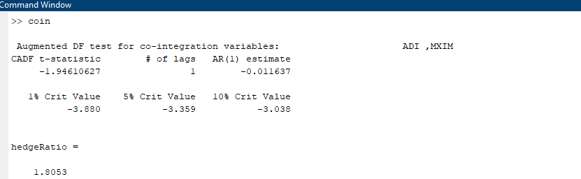
    The t-statistic of this test is – 1.9416 which is way lesser than the 90% threshold and we can safely assume that this pair is NOT cointegrated. The hedge ratio is 1.8053 but this does not seem to be a good candidate for pairs trading. Going based on correlation alone would have been the wrong move!


    Now, let’s look at two other stocks ( SPY and QCOM) again over the past 3 years and run the same cointegration test.


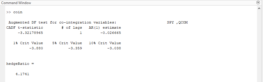
    As you can see the t-statistic is a much better -3.3217 which implies a more than 90% probability that the two time series are co-integrated. This would need more validation before putting on the trade at a hedge ratio of 4.174 but definitely seems more promising than the previous pair. 

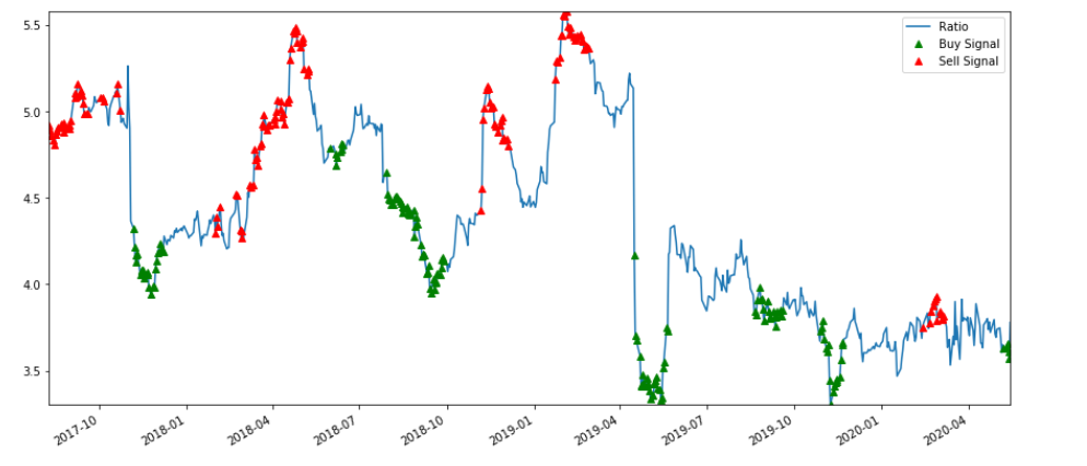
    I will not go into generating specific trading signals because that exercise is very nuanced and there are several attributes to consider including training/testing the data set and specific signaling algorithms. However, as a very simplistic illustration, the chart below indicates the z-score based buy and sell signals for the SPY/QCOM pair based on the assumption that the ratio reverts to the mean. The trading signals are generated from a measure of the rolling mean (60 day Moving Average) and (60 day standard deviation). The z score is (5 day moving average – 60 day moving average) divided by (60 day standard deviation).  Though this set up looks promising, this needs to be validated further.


    All that said, keep in mind that:

    1) When regime shifts occur the past data may not absolutely indicate what will happen in the future. 

    2) If there are obvious pair trading combos, the arbitrageurs will be at work minimizing the marginal utility of the idea. 

    3) The other basic assumption underlying the algo is that the financial data is normally distributed ( in reality however financial data may not be normally distributed and may exhibit fat tail behavior).

    4) Don’t be wed to any strategy and refrain from picking data points to prove a preconceived notion. If testing on in sample and out sample data sets do not provide statistically significant and consistent results, it is probably telling you to not rely on the strategy.

    5) There is beauty in simplicity. Keep the model and algorithm as uncomplicated as possible.

    Notwithstanding the above,  an appreciation of the data and underlying math can help effectively structure your code and increase your odds of success; as long as you don’t throw risk management out of the window.